Theory: Thermal Hydraulics
Nodalization
The thermal-hydraulic model is built from single-node or multi-node 1D pipes connected by junctions. Internal junctions are automatically generated for multi-node pipes. See Two single-node pipes A and B connected by a junction o.
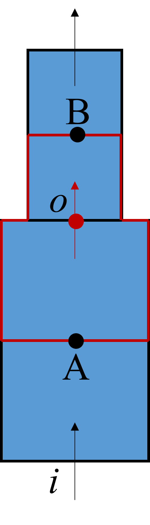
Two single-node pipes \(A\) and \(B\) connected by a junction \(o\)
Pipes can be of different types as described in input description:
pipe-f : Pipe with free level (always single-node)
pipe-t : Pipe without free level with temperature defined by signal (always single-node)
The simulated circuit should be a closed network of 1D pipes, including at least one single-node pipe with a free surface. The gas pressure above the free surface is a boundary condition for the model. See Example of the closed network.
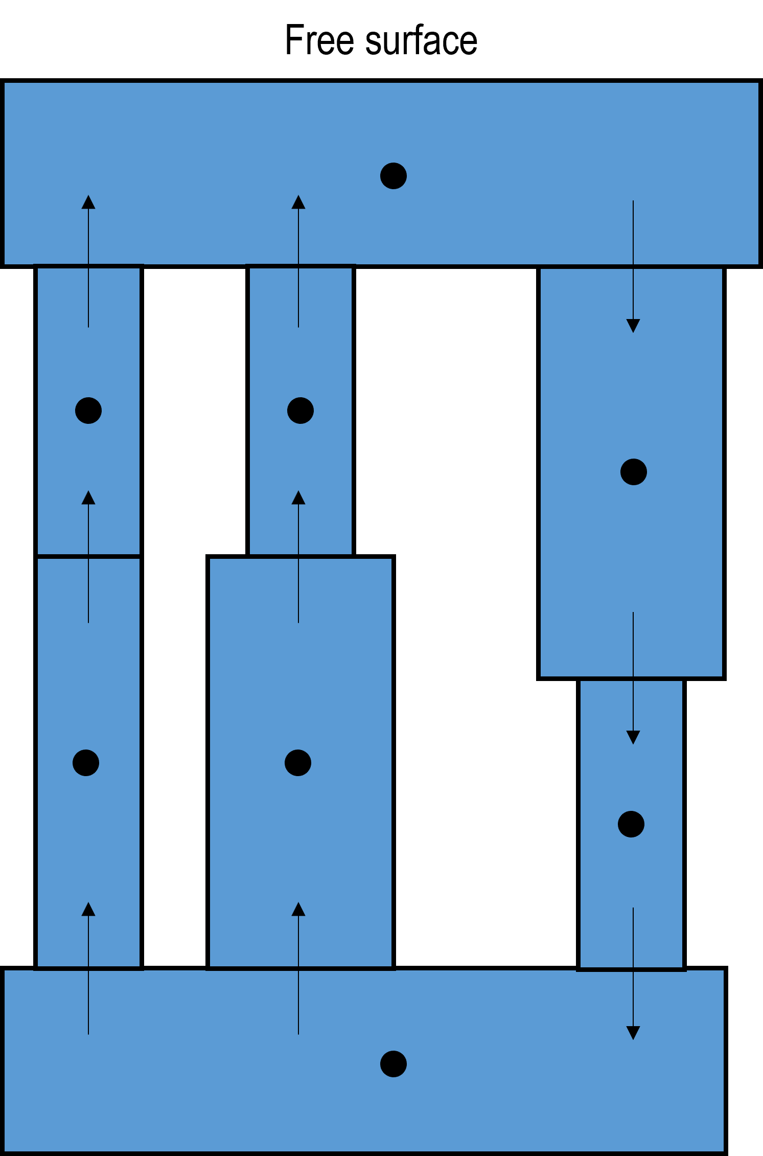
Example of the closed network
Main equations
A 1D single-phase thermal-hydraulic model of ROOSTER for a non-compressible fluid includes
liquid sodium and liquid lead equations-of-state;
mass conservation equation (1);
momentum conservation equation (2);
energy conservation equation (3).
Mass conservation equation
Mass conservation equation is written for every node. See Two single-node pipes A and B connected by a junction o.
where
\[\sum_{in} G_i\]
|
the sum of mass flowrates over the inlet junctions of the node |
kg/s |
\[\sum_{out} G_o\]
|
the sum of mass flowrates over the outlet junctions of the node |
kg/s |
Momentum conservation equation
Momentum conservation equation is written for every junction, e.g. junction \(o\), connecting the nodes \(A\) and \(B\). See Two single-node pipes A and B connected by a junction o.
where
\(L_A\) and \(L_B\) |
the lengths of nodes A and B |
m |
\(A_A\) and \(A_B\) |
the flow areas of nodes A and B |
m2 |
\(G_o\) |
the flowrate in junction o |
kg/s |
\(P_A\) and \(P_B\) |
the pressure in nodes A and B |
Pa |
\({\rho}\) |
the coolant density |
kg/ m3 |
\({v}\) |
the velocity |
m/s |
\(\Delta P_{GRAV} = ( \rho g H/2 )_A + ( \rho g H/2 )_B\) |
gravity head |
Pa |
\(g\) |
the acceleration due to gravity |
m/s2 |
\(H\) |
the elevation of the node |
m |
\(\Delta P_{FRIC}\) |
the friction loss |
Pa |
\(\Delta P_{PUMP}\) |
the pump head |
Pa |
Energy conservation equation
Energy conservation equation is written for every node. See Two single-node pipes A and B connected by a junction o.
where
\({\rho}\) |
the coolant density in the node |
kg/ m3 |
\(v\) |
the coolant velocity in the node |
m/s |
\(h\) |
the coolant specific enthalpy in the node |
J/kg |
\(t\) |
the time |
s |
\(G_i\) |
the flowrate in the inlet junction \(i\) |
kg/s |
\(h_i\) |
the coolant specific enthalpy in the inlet junction \(i\) |
J/kg |
\[\sum_{in}\]
|
the sum of mass flowrates over the inlet junctions of the node |
|
\(G_o\) |
the flowrate in the outlet junction \(o\) |
kg/s |
\(h_o\) |
the coolant specific enthalpy in the outlet junction \(o\) |
J/kg |
\[\sum_{out}\]
|
the sum of mass flowrates over the outlet junctions of the node |
|
\(q_w\) |
the heat flux from all heat exchange surfaces in the node |
W/m2 |
\(A_w\) |
the area of all heat exchange surfaces in the node |
m2 |
Algorithm for finding pressure
The algorithm for finding pressure is as follows:
A set of linear algebraic equations is built of
mass conservation equations (1) written for every node (except nodes of the pipes with a free surface) and differentiated with respect to time so that left-hand sides are sum of time derivatives of inlet and outlet mass flowrates and right-hand sides are zeros:
(4)\[\sum_{in} \frac{dG_i}{dt} - \sum_{out} \frac{dG_o}{dt} = 0\]momentum conservation equations for every junction between the nodes so that left-hand sides are time derivatives of mass flowrate in the junctions and differences of the pressures in two nodes connected by the junction, while right-hand sides are gravity heads, friction pressure losses and momentum sources.
The set of linear algebraic equations is solved with respect to time derivatives of momentum in every junction and pressure values in every node.
Time integration
The time derivatives of mass flowrate in junctions and enthalpies in nodes are then integrated using an ODE solver LSODES available from the SciPy library .
Closure relations
The closure relations of the model includes
correlations for friction factors
the Rehme model for tube bundles [Rehme1973] and
the Churchill model for pipes [Churchill1977]
correlations for heat exchange coefficient
the Mikityuk model [Mikityuk2009] for tube bundles and
the Subbotin correlation for pipes [Subbotin1962].